IT in Geophysics - Classifying Earth from above with Machine Learning

Humanity has found a way to analyze almost every aspect of the earth using maps. We have been able to visualize climate change, de/reforestation, city growth, etc. using satellite images. How are these maps created and how can we show all these important aspects of the earth so well? In this article, we will dabble into the world of remote sensing and how machine learning algorithms help us classify geothermic images.

Remote sensing is exclusively possible because of electromagnetic radiation. Electromagnetic radiation is made up of electrically charged particles called photons, which are the fundamental units of light. These photons can be exhibited as both a wave and a particle. The wavelength of a photon is related to its energy through the equation E = (h*c)/λ, where E is the energy of the photon, h is the Planck constant, c is the speed of light, and λ is the wavelength of the photon. This equation shows that the shorter the wavelength, the higher the energy of the photon.

Absorption and scattering are two important phenomena that can be described when identifying a photon as a particle. Absorption occurs when a photon is absorbed by an atom or molecule and its energy is transferred to the atom or molecule. Scattering occurs when a photon is deflected by an atom or molecule and changes direction.

Due to scattering we can see colors, as some wavelengths are visible for the human eye. For example, leaves are usually green, since they scatter photons with a wavelength that represents green. The visible light spectrum is only a very small part of all the possible wavelengths identified on earth.

Image classification

These phenomena are used in remote sensing to create maps from satellite images. This process involves collecting images of the Earth’s surface from satellites or other aerial platforms and then using these images to create maps. The images are typically taken in different wavelengths of the electromagnetic spectrum so called ‘bands’, such as visible light or infrared, and can provide a wide range of information about the Earth’s surface, including its composition, topography, and land cover. For example, if a researcher wishes to analyze vegetation growth, the best way to separate the trees from other objects is to use the near-infrared and red bands. Healthy vegetation usually has a high reflectance in the near-infrared band and low reflectance in the red band.

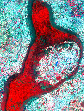
This is what is shown in Figure 1. It looks really interesting, but why is this done and how does this go from a very detailed image, to a very simplistic, easy to understand map? Luckily, machine learning algorithms known as “Image Analysis Methods” help us classify these images to single-colored pixels.

Image Analysis Methods

The process of classifying an image does take some human effort. A user first ‘trains’ the algorithm by classifying small areas of a certain class. For example in Figure 1, we could have two classes; forest and no forest. An important question to ask is: how is it possible to differentiate forests with other vegetation?
Different land covers sometimes do reflect the same color, but we have various means of differentiating them, such as texture, shape, size, pattern, etc. In our context, forests have a more grainy texture, whereas other vegetation, such as fields, have a smooth texture. Therefore, we will classify grainy, reddish areas as ‘forest’ and other areas as ‘no forest’. After the initial classification is finished, an algorithm will be chosen to further classify this image. Figure 2 shows the final product.

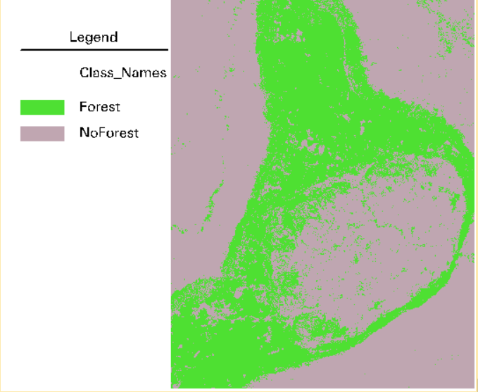
Figure 2 is classified using an algorithm called Random Forest (RF). No, this name does not come from being able to classify forests with it, but because it splits the data into subsets and uses the ‘majority vote’ of multiple decision trees to classify pixels. Compared to a single decision tree algorithm, it greatly reduces its overfitting problem by doing this. Its namepart ‘random’ stems from the fact that the decision trees are created randomly. Another positive of RF, is that its parameters are comparatively found to be very robust.
On the other hand, RF-classification may have difficulties handling very large datasets. This is not a problem for Support Vector Machines (SVMs), which is another machine learning algorithm. They can handle large datasets very efficiently. Additionally, it can handle very small datasets with good accuracy as well. Just like RF, SVM has a small chance of overfitting, as it uses a hyperplane in a feature space, ignoring outliers. Although this lightweight algorithm works very efficiently, it cannot reach an accuracy as high as other popular algorithms in remote sensing.

Another very accurate machine learning algorithm used in remote sensing is Convolutional Neural Networks (CNNs). As opposed to previous shallow algorithms, CNNs deep learning allows it to have a better and more powerful generalization ability than other algorithms. Sadly, due to the limited amount of training data in the field, CNN is not able to live up to its potential. Additionally, compared to others, it has a very high computational cost and thus has a very low time efficiency as of now.

These algorithms all have something in common, which is the fact that they are pixel-based, meaning that they classify each pixel as a certain class. Another method of classifying remote sensing images is Object Based Image Analysis (OBIA). OBIA is a fairly new found method that involves grouping pixels into ‘objects’ based on their physical properties, rather than analyzing individual pixels in isolation. These objects can be individual buildings, trees, or other features on the ground.

One advantage of OBIA is that it can more accurately capture the shape, size, and context of features on the ground, since it takes into account the relationships between pixels within an object. This can be particularly useful for detecting and mapping features that are difficult to discern at the pixel level, such as small buildings or trees. Another advantage of OBIA is that it can more effectively incorporate additional sources of information, such as topographic data or prior knowledge about the landscape, to improve the accuracy of the analysis.
However, there are also some disadvantages to OBIA.

One disadvantage is that it can be more computationally intensive than pixel-based algorithms, since it involves analyzing and grouping large numbers of pixels into objects. Additionally, OBIA can be more sensitive to changes in the resolution or quality of the imagery, since it relies on the relationships between pixels within an object.

Conclusion

As in other fields, there is more than one viable algorithm to set your heart on. It is not as simple as picking the best algorithm, as it does not exist. Every algorithm has its advantages and disadvantages. The art of choosing the most applicable algorithm relies on the dataset available, or just trying every algorithm there is. The choice is up to you.

References

https://www.tandfonline.com/doi/full/10.1080/01431161.2018.1433343
https://arxiv.org/abs/1508.00092
https://www.tandfonline.com/doi/full/10.1080/20964471.2019.1657720
https://link.springer.com/chapter/10.1007/978-3-540-77058-9_1
https://www.sciencedirect.com/science/article/pii/S0924271613002220